Time-dependent operators
This tutorial explains how to define time-dependent Hamiltonians – and more generally time-dependent operators – in Dynamiqs. There are currently four supported formats: constant operator, piecewise constant operator, constant operator modulated by a time-dependent factor, or arbitrary time-dependent operator defined by a function.
import dynamiqs as dq
import jax.numpy as jnp
from matplotlib import pyplot as plt

dq.plot.mplstyle(dpi=150)  # set custom matplotlib style
The TimeQArray type
In Dynamiqs, time-dependent operators are defined with type TimeQArray. They can be called at arbitrary times, and return the corresponding qarray at that time. For example to define the Hamiltonian
$$
H_x(t)=\cos(2\pi t)\sigma_x
$$
>>> f = lambda t: jnp.cos(2.0 * jnp.pi * t)
>>> Hx = dq.modulated(f, dq.sigmax())  # initialize a modulated timeqarray
>>> Hx(1.0)
QArray: shape=(2, 2), dims=(2,), dtype=complex64, layout=dia, ndiags=2
[[  ⋅    1.+0.j]
 [1.+0.j   ⋅   ]]
>>> Hx.shape
(2, 2)
Timeqarrays support common arithmetic operations with scalars, qarray-likes and other timeqarrays. For example to define the Hamiltonian $$ H(t) = \sigma_z + 2 H_x(t) - \sin(\pi t) \sigma_y $$
>>> g = lambda t: jnp.sin(jnp.pi * t)
>>> Hy = dq.modulated(g, dq.sigmay())
>>> H = dq.sigmaz() + 2 * Hx - Hy
>>> H(1.0)
QArray: shape=(2, 2), dims=(2,), dtype=complex64, layout=dia, ndiags=3
[[ 1.+0.j  2.-0.j]
 [ 2.+0.j -1.+0.j]]
Finally, timeqarrays also support common utility functions, such as .conj(), or .reshape(). More details can be found in the TimeQArray API page.
Defining a timeqarray
Constant operators
A constant operator is defined by
$$
O(t) = O_0
$$
for any time \(t\), where \(O_0\) is an arbitrary operator. The most practical way to define constant operators is using qarray-likes. They can also be instantiated as timeqarrays using the dq.constant() function. For instance, to define the Pauli operator \(H = \sigma_z\), you can use any of the following syntaxes:
import dynamiqs as dq
H = dq.sigmaz()
import dynamiqs as dq
H = dq.asqarray([[1, 0], [0, -1]])
import numpy as np
H = np.array([[1, 0], [0, -1]])
import jax.numpy as jnp
H = jnp.array([[1, 0], [0, -1]])
import qutip as qt
H = qt.sigmaz()
H = [[1, 0], [0, -1]]
Note
Common operators are available as utility functions, see the list of available operators in the Python API.
Piecewise constant operators
A piecewise constant (PWC) operator takes constant values over some time intervals. It is defined by $$ O(t) = \left(\sum_{k=0}^{N-1} c_k\; \Omega_{[t_k, t_{k+1}[}(t)\right) O_0 $$ where \(c_k\) are constant values, \(\Omega_{[t_k, t_{k+1}[}\) is the rectangular window function defined by \(\Omega_{[t_a, t_b[}(t) = 1\) if \(t \in [t_a, t_b[\) and \(\Omega_{[t_a, t_b[}(t) = 0\) otherwise, and \(O_0\) is a constant operator.
In Dynamiqs, PWC operators are defined by:
times: the time points \((t_0, \ldots, t_N)\) defining the boundaries of the time intervals, of shape (N+1,),values: the constant values \((c_0, \ldots, c_{N-1})\) for each time interval, of shape (..., N),qarray: the qarray defining the constant operator \(O_0\), of shape (n, n).
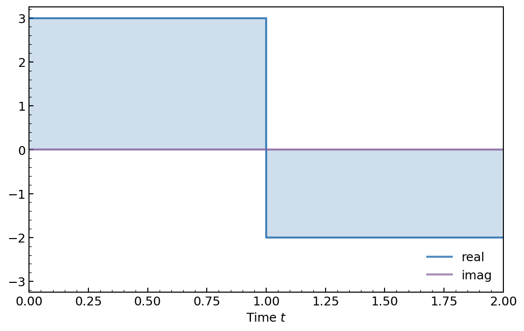
To construct a PWC operator, these three arguments must be passed to the dq.pwc() function, which returns a timeqarray. When called at some time \(t\), this object then returns a qarray with shape (..., n, n). For example, let us define a PWC operator \(H(t)\) with constant value \(3\sigma_z\) for \(t\in[0, 1[\) and \(-2\sigma_z\) for \(t\in[1, 2[\):
>>> times = [0.0, 1.0, 2.0]
>>> values = [3.0, -2.0]
>>> qarray = dq.sigmaz()
>>> H = dq.pwc(times, values, qarray)
>>> H
PWCTimeQArray: shape=(2, 2), dims=(2,), dtype=complex64, layout=dia, ndiags=1
The returned object can be called at different times:
>>> H(-1.0)
QArray: shape=(2, 2), dims=(2,), dtype=complex64, layout=dia, ndiags=1
[[  ⋅      ⋅   ]
 [  ⋅      ⋅   ]]
>>> H(0.0)
QArray: shape=(2, 2), dims=(2,), dtype=complex64, layout=dia, ndiags=1
[[ 3.+0.j    ⋅   ]
 [   ⋅    -3.+0.j]]
>>> H(0.5)
QArray: shape=(2, 2), dims=(2,), dtype=complex64, layout=dia, ndiags=1
[[ 3.+0.j    ⋅   ]
 [   ⋅    -3.+0.j]]
>>> H(1.0)
QArray: shape=(2, 2), dims=(2,), dtype=complex64, layout=dia, ndiags=1
[[-2.+0.j    ⋅   ]
 [   ⋅     2.+0.j]]
>>> H(1.5)
QArray: shape=(2, 2), dims=(2,), dtype=complex64, layout=dia, ndiags=1
[[-2.+0.j    ⋅   ]
 [   ⋅     2.+0.j]]
>>> H(2.0)
QArray: shape=(2, 2), dims=(2,), dtype=complex64, layout=dia, ndiags=1
[[  ⋅      ⋅   ]
 [  ⋅      ⋅   ]]
We can use dq.plot.pwc_pulse() to plot the PWC pulse values at different times:
dq.plot.pwc_pulse(H.times, H.values)
plt.gca().set(xlabel='Time $t$')
Note
The argument times must be sorted in ascending order, but does not need to be evenly spaced. When calling the resulting timeqarray at time \(t\), the returned qarray is the operator \(c_k\ O_0\) corresponding to the interval \([t_k, t_{k+1}[\) in which the time \(t\) falls. If \(t\) does not belong to any time intervals, the returned qarray is null.
Batching PWC operators
The batching of the returned timeqarray is specified by values. For example, to define a PWC operator batched over a parameter \(\theta\):
>>> thetas = jnp.linspace(0, 1.0, 11)  # (11,)
>>> times = [0.0, 1.0, 2.0]
>>> values = thetas[:, None] * jnp.array([3.0, -2.0])  # (11, 2)
>>> qarray = dq.sigmaz()
>>> H = dq.pwc(times, values, qarray)
>>> H.shape
(11, 2, 2)
Modulated operators
A modulated operator is defined by $$ O(t) = f(t) O_0 $$ where \(f(t)\) is a time-dependent scalar. In Dynamiqs, modulated operators are defined by:
f: a Python function with signaturef(t: float) -> Scalar | Arraythat returns the modulating factor \(f(t)\) for any time \(t\), as a scalar or an array of shape (...),qarray: the qarray defining the constant operator \(O_0\), of shape (n, n).
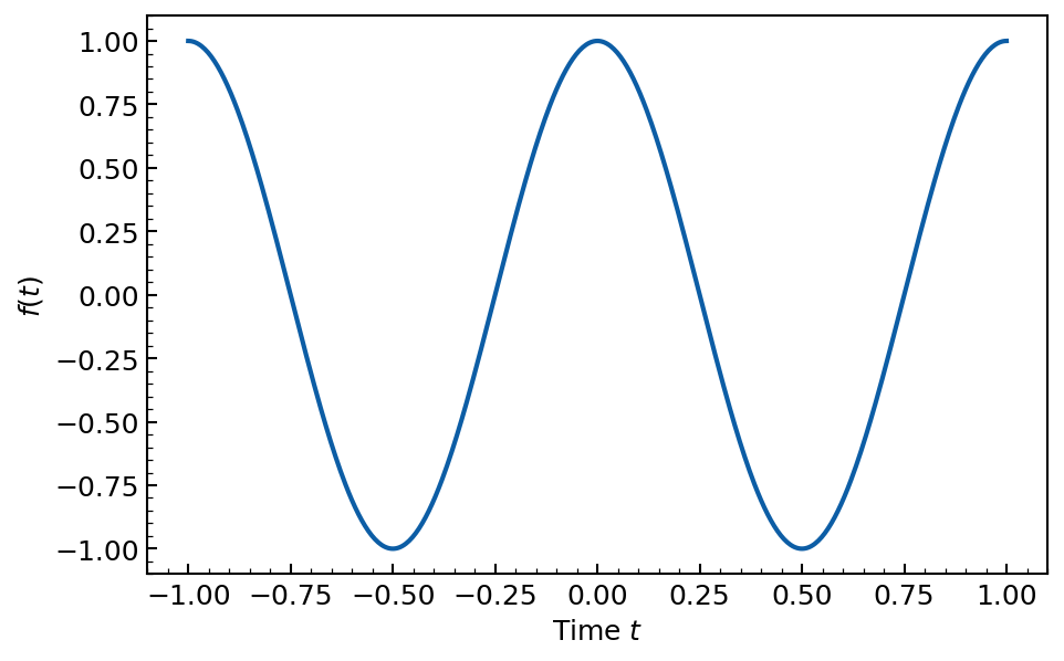
To construct a modulated operator, these two arguments must be passed to the dq.modulated() function, which returns a timeqarray. When called at some time \(t\), this object then returns a qarray with shape (..., n, n). For example, let us define the modulated operator \(H(t)=\cos(2\pi t)\sigma_x\):
>>> f = lambda t: jnp.cos(2.0 * jnp.pi * t)
>>> H = dq.modulated(f, dq.sigmax())
>>> H
ModulatedTimeQArray: shape=(2, 2), dims=(2,), dtype=complex64, layout=dia, ndiags=2
The returned object can be called at different times:
>>> H(0.5)
QArray: shape=(2, 2), dims=(2,), dtype=complex64, layout=dia, ndiags=2
[[   ⋅    -1.+0.j]
 [-1.+0.j    ⋅   ]]
>>> H(1.0)
QArray: shape=(2, 2), dims=(2,), dtype=complex64, layout=dia, ndiags=2
[[  ⋅    1.+0.j]
 [1.+0.j   ⋅   ]]
We can use the prefactor() method to plot \(f(t)\) at different times:
ts = jnp.linspace(-1.0, 1.0, 501)
plt.plot(ts, H.prefactor(ts))
plt.gca().set(xlabel='Time $t$', ylabel='$f(t)$')
Batching modulated operators
The batching of the returned timeqarray is specified by the array returned by f. For example, to define a modulated Hamiltonian \(H(t)=\cos(\omega t)\sigma_x\) batched over the parameter \(\omega\):
>>> omegas = jnp.linspace(0.0, 1.0, 11)  # (11,)
>>> f = lambda t: jnp.cos(omegas * t)
>>> H = dq.modulated(f, dq.sigmax())
>>> H.shape
(11, 2, 2)
Function with additional arguments
To define a modulated operator with a function that takes arguments other than time (extra *args and **kwargs), you can use functools.partial(). For example:
>>> import functools
>>> def pulse(t, omega, amplitude=1.0):
...     return amplitude * jnp.cos(omega * t)
>>> # create function with correct signature (t: float) -> Array
>>> f = functools.partial(pulse, omega=1.0, amplitude=5.0)
>>> H = dq.modulated(f, dq.sigmax())
Discontinuous function
If there is a discontinuous jump in the function values, you should use the optional
argument discontinuity_ts to enforce adaptive step size methods to stop at these
times (i.e., right before, and right after the jump).
Arbitrary time-dependent operators
An arbitrary time-dependent operator is defined by $$ O(t) = f(t) $$ where \(f(t)\) is a time-dependent operator. In Dynamiqs, arbitrary time-dependent operators are defined by:
f: a Python function with signaturef(t: float) -> QArraythat returns the operator \(f(t)\) for any time \(t\), as a qarray of shape (..., n, n).
To construct an arbitrary time-dependent operator, pass this argument to the dq.timecallable() function, which returns a timeqarray. This object then returns a qarray with shape (..., n, n) when called at any time \(t\).
For example, let us define the arbitrary time-dependent operator \(H(t)=\begin{pmatrix}t & 0\\0 & 1 - t\end{pmatrix}\):
>>> f = lambda t: dq.asqarray([[t, 0], [0, 1 - t]])
>>> H = dq.timecallable(f)
>>> H
CallableTimeQArray: shape=(2, 2), dims=(2,), dtype=float32, layout=dense
The returned object can be called at different times:
>>> H(0.5)
QArray: shape=(2, 2), dims=(2,), dtype=float32, layout=dense
[[0.5 0. ]
 [0.  0.5]]
>>> H(1.0)
QArray: shape=(2, 2), dims=(2,), dtype=float32, layout=dense
[[1. 0.]
 [0. 0.]]
The function f must return a qarray (not a qarray-like!)
An error is raised if the function f does not return a qarray. This error concerns any other qarray-likes. This is enforced to avoid costly conversions at every time step of the numerical integration.
Batching arbitrary time-dependent operators
The batching of the returned timeqarray is specified by the qarray returned by f. For example, to define an arbitrary time-dependent operator batched over a parameter \(\theta\):
>>> thetas = jnp.linspace(0, 1.0, 11)  # (11,)
>>> f = lambda t: thetas[:, None, None] * dq.asqarray([[t, 0], [0, 1 - t]])
>>> H = dq.timecallable(f)
>>> H.shape
(11, 2, 2)
Function with additional arguments
To define an arbitrary time-dependent operator with a function that takes arguments other than time (extra *args and **kwargs), you can use functools.partial(). For example:
>>> import functools
>>> def func(t, a, amplitude=1.0):
...     return amplitude * dq.asqarray([[t, a], [a, 1 - t]])
>>> # create function with correct signature (t: float) -> Array
>>> f = functools.partial(func, a=1.0, amplitude=5.0)
>>> H = dq.timecallable(f)
Discontinuous function
If there is a discontinuous jump in the function values, you should use the optional
argument discontinuity_ts to enforce adaptive step size methods to stop at these
times (i.e., right before, and right after the jump).
Clipping a timeqarray
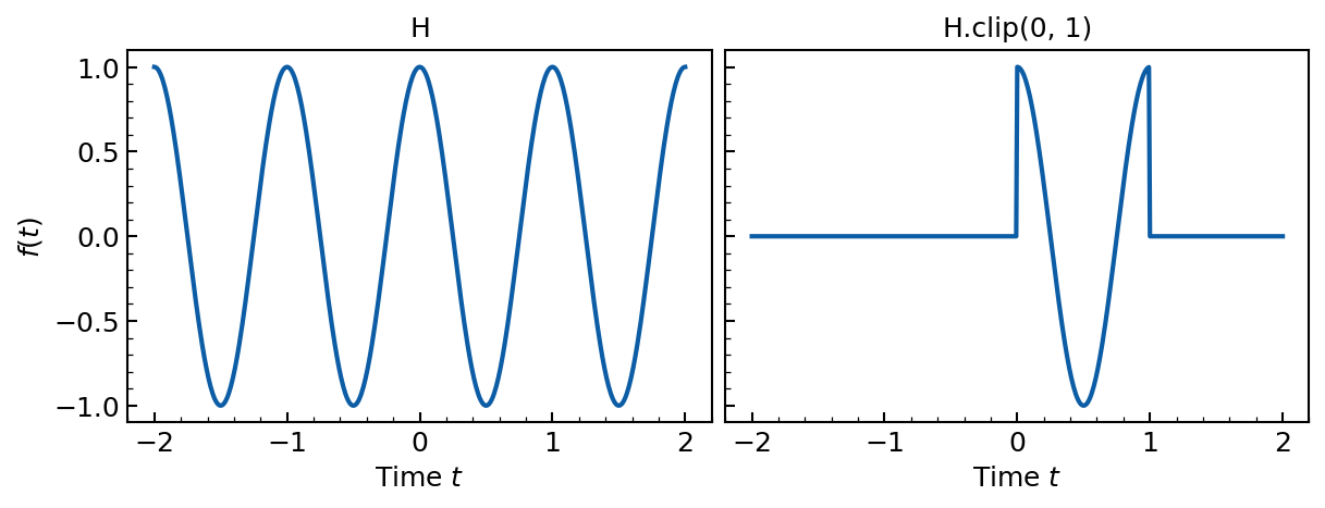
Time-dependent operators can be clipped to a given time interval, outside which the returned qarray is null. For example:
>>> f = lambda t: jnp.cos(2.0 * jnp.pi * t)
>>> H = dq.modulated(f, dq.sigmax())
>>> H(2.0)
QArray: shape=(2, 2), dims=(2,), dtype=complex64, layout=dia, ndiags=2
[[  ⋅    1.+0.j]
 [1.+0.j   ⋅   ]]
>>> H_clipped = H.clip(0, 1)  # clip to 0 <= t < 1
>>> H_clipped(2.0)
QArray: shape=(2, 2), dims=(2,), dtype=complex64, layout=dia, ndiags=2
[[  ⋅      ⋅   ]
 [  ⋅      ⋅   ]]
We can plot the resulting prefactor values after clipping:
_, axs = dq.plot.grid(2, w=4, h=3, sharexy=True)
ax0, ax1 = list(axs)

ts = jnp.linspace(-2.0, 2.0, 501)

ax0.plot(ts, H.prefactor(ts))
ax0.set(xlabel='Time $t$', ylabel='$f(t)$', title='H')

ax1.plot(ts, H_clipped.prefactor(ts))
ax1.set(xlabel='Time $t$', title='H.clip(0, 1)')
Shifting a timeqarray
You can shift the time dependence of any timeqarray without redefining it. A shifted
timeqarray is defined by
$$
O_{\text{shift}}(t) = O(t - t_{\text{shift}}).
$$
Use the .shift() method:
>>> f = lambda t: jnp.cos(2.0 * jnp.pi * t)
>>> H = dq.modulated(f, dq.sigmax())
>>> H_shift = H.shift(0.5)
>>> H_shift(0.0) # == H(0.5)
QArray: shape=(2, 2), dims=(2,), dtype=complex64, layout=dia, ndiags=2
[[   ⋅    -1.+0.j]
 [-1.+0.j    ⋅   ]]
>>> H(0.5)
QArray: shape=(2, 2), dims=(2,), dtype=complex64, layout=dia, ndiags=2
[[   ⋅    -1.+0.j]
 [-1.+0.j    ⋅   ]]
If the timeqarray is clipped, shifting it also moves the clipping window by the same amount. We can visualize the effect of shifting a clipped timeqarray:
H_clipped_shift = H.clip(0, 1).shift(0.5)

_, axs = dq.plot.grid(3, w=5, h=4, sharexy=True)
ax0, ax1, ax2 = list(axs)

ts = jnp.linspace(-1.0, 2.5, 501)

ax0.plot(ts, H.prefactor(ts))
ax0.set(ylabel='$f(t)$', title='H')

ax1.plot(ts, H_shift.prefactor(ts))
ax1.set(title='H.shift(0.5)')

ax2.plot(ts, H_clipped_shift.prefactor(ts))
ax2.set(xlabel='Time $t$', title='H.clip(0, 1).shift(0.5)')


