Continuous jump measurement
Work in progress.
This tutorial is under construction, this is a draft version.
In this example, we simulate stochastic trajectories of quantum systems that are continuously measured by a jump detector. We explain how to use dq.jssesolve() to simulate trajectories modelled by the jump SSE, and dq.jsmesolve() to simulate trajectories modelled by the jump SME.
import jax
import jax.numpy as jnp
import numpy as np
from matplotlib import pyplot as plt
import dynamiqs as dq

dq.plot.mplstyle(dpi=150)  # set custom matplotlib style
Qubit
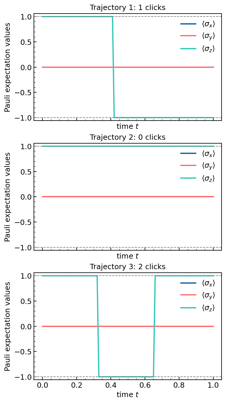
We consider a qubit starting from \(\ket{\psi_0}=\ket1\), with no unitary dynamic \(H=0\) and two loss operators \(L_-=\sigma_-\) and \(L_+=\sigma_+\) which are continuously measured by jump detectors. We expect stochastic trajectories jumping between the excited and ground state.
Let's begin with a perfectly efficient detector. We start with a pure state, and we measure all loss channels with perfect efficiency, so we don't loose any information about the system's state. As a result, it remains pure at all times. We use dq.jssesolve() to simulate these quantum trajectories.
Simulation
# define Hamiltonian, jump operators, initial state
H = dq.zeros(2)
jump_ops = [dq.sigmam(), dq.sigmap()]
psi0 = dq.excited()

# define save times
tsave = np.linspace(0, 2.0, 101)

# define a certain number of PRNG key, one for each trajectory
key = jax.random.PRNGKey(42)
ntrajs = 3
keys = jax.random.split(key, ntrajs)

# simulate trajectories
method = dq.method.EulerJump(dt=1e-3)
result = dq.jssesolve(H, jump_ops, psi0, tsave, keys, method=method)
print(result)
==== JSSESolveResult ====
Method     : EulerJump
Infos      : 1000 steps | infos shape (3,)
States     : QArray complex64 (3, 101, 2, 1) | 7.9 Kb
Clicktimes : Array float32 (3, 2, 10000) | 390.6 Kb
>>> result.states.shape  # (ntrajs, ntsave, n, 1)
(3, 101, 2, 1)
>>> result.clicktimes.shape  # (ntrajs, nLm, nmaxclick)
(3, 2, 10000)
Individual state trajectories
_, axs = dq.plot.grid(ntrajs, ntrajs, w=5, h=3, sharexy=True)

for i in range(ntrajs):
    ax = next(axs)
    dq.plot.xyz(result.states[i], times=tsave, ax=ax)
    ax.set(
        title=f'Trajectory {i+1}: {result.nclicks[i].sum()} clicks',
        xlabel=r'time $t$',
        ylabel='Pauli expectation values',
    )
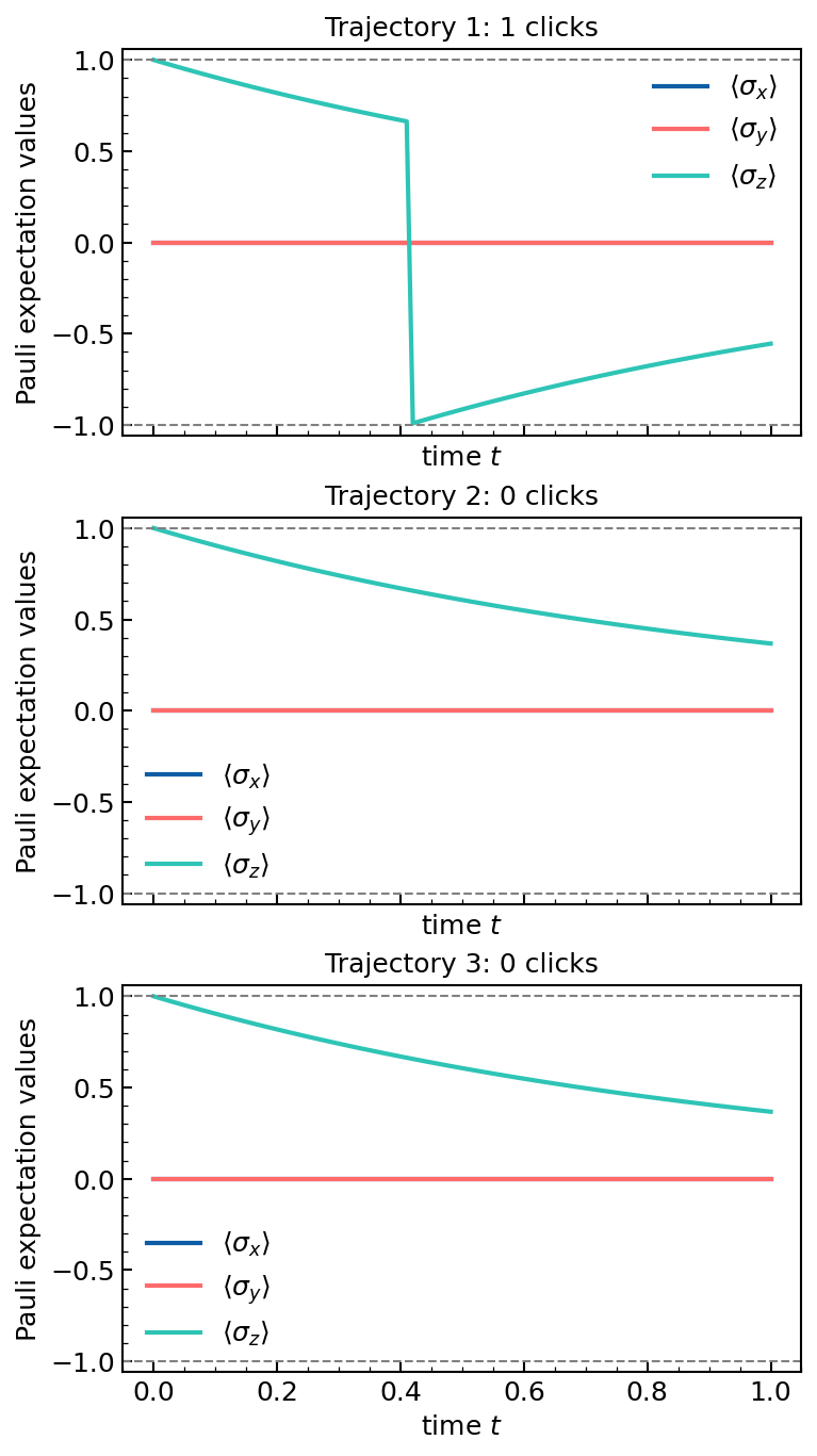
Imperfect detection
If the detection is imperfect, the system state is a density matrix. We use dq.jsmesolve() to simulate these quantum trajectories. For jump measurement we can model two classes of imperfections: false clicks (accounted by the dark count rate \(\theta\)) and missed clicks (accounted by the efficiency \(\eta\)).
# define dark count rates
thetas = [0.0, 0.0]
# define efficiencies
etas = [0.5, 0.5]

# simulate trajectories
result = dq.jsmesolve(H, jump_ops, thetas, etas, psi0, tsave, keys, method=method)
print(result)
==== JSMESolveResult ====
Method     : EulerJump
Infos      : 1000 steps | infos shape (3,)
States     : QArray complex64 (3, 101, 2, 2) | 9.5 Kb
Clicktimes : Array float32 (3, 2, 10000) | 234.4 Kb
>>> result.states.shape  # (ntrajs, ntsave, n, n)
(3, 101, 2, 2)
>>> result.clicktimes.shape  # (ntrajs, nLm, nmaxclick)
(3, 2, 10000)
_, axs = dq.plot.grid(ntrajs, ntrajs, w=5, h=3, sharexy=True)

for i in range(ntrajs):
    ax = next(axs)
    dq.plot.xyz(result.states[i], times=tsave, ax=ax)
    ax.set(
        title=f'Trajectory {i+1}: {result.nclicks[i].sum()} clicks',
        xlabel=r'time $t$',
        ylabel='Pauli expectation values',
    )
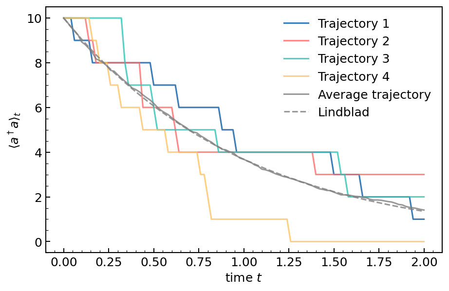
Quantum harmonic oscillator
We consider a quantum harmonic oscillator starting from the Fock state \(\ket{n_0}\), with Hamiltonian \(H=0\) and a single loss operator \(L=\sqrt\kappa a\) which is continuously measured by photodetection.
Simulation
# define Hamiltonian, jump operators, initial state
n = 16
a = dq.destroy(n)
kappa = 1.0
n0 = 10
H = dq.zeros(n)
jump_ops = [jnp.sqrt(kappa) * a]
psi0 = dq.fock(n, n0)

# define save times
tsave = np.linspace(0, 2.0, 101)

# define a certain number of PRNG key, one for each trajectory
key = jax.random.PRNGKey(42)
ntrajs = 100
keys = jax.random.split(key, ntrajs)

# simulate trajectories
method = dq.method.EulerJump(dt=1e-3)
exp_ops = [a.dag() @ a]
result = dq.jssesolve(H, jump_ops, psi0, tsave, keys, method=method, save_states=False, exp_ops=exp_ops)
print(result)
==== JSMESolveResult ====
Method     : EulerJump
Infos      : 1000 steps | infos shape (1000,)
States     : QArray complex64 (100, 16, 1) | 2.0 Mb
Expects    : Array complex64 (100, 1, 101) | 789.1 Kb
Clicktimes : Array float32 (100, 1, 10000) | 38.1 Mb
Individual trajectories vs average trajectory vs Lindblad solution
exps_adaga = result.expects[:, 0, :].real
kw = dict(lw=1.5, alpha=0.8)

# individual trajectories
for i, exp in enumerate(exps_adaga[:4]):
    plt.plot(tsave, exp, label=f'Trajectory {i+1}', **kw)

# average trajectory
plt.plot(tsave, exps_adaga.mean(0), label=f'Average trajectory', color='gray', **kw)

# Lindblad solution
result_lindblad = dq.mesolve(H, jump_ops, psi0, tsave, save_states=False, exp_ops=exp_ops)
plt.plot(tsave, result_lindblad.expects[0].real, ls='--', label=f'Lindblad', color='gray', **kw)

plt.gca().set(
    xlabel=r'time $t$',
    ylabel=r'$\langle a^\dagger a \rangle_t$',
)
plt.legend()