fock

fock

fock.fock

fock(
    state: QArrayLike,
    *,
    ax: Axes | None = None,
    allxticks: bool = False,
    ymax: float | None = 1.0,
    color: str = colors["blue"],
    alpha: float = 1.0,
    label: str = ""
)

Plot the photon number population of a state.

Warning

Documentation redaction in progress.

Examples

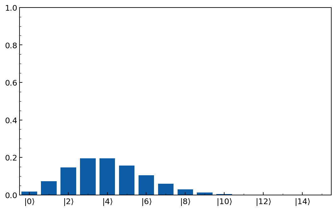
>>> psi = dq.coherent(16, 2.0)
>>> dq.plot.fock(psi)

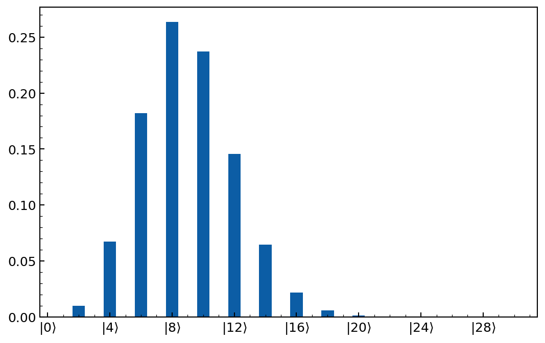
>>> # the even cat state has only even photon number components
>>> psi = (dq.coherent(32, 3.0) + dq.coherent(32, -3.0)).unit()
>>> dq.plot.fock(psi, allxticks=False, ymax=None)

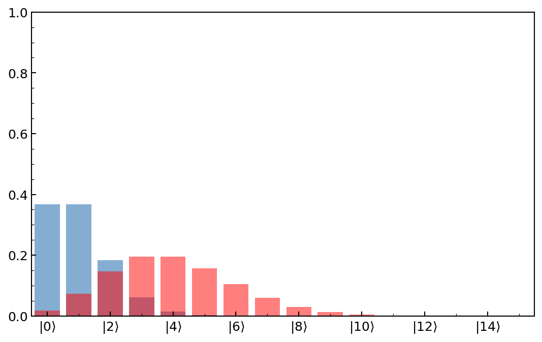
>>> dq.plot.fock(dq.coherent(16, 1.0), alpha=0.5)
>>> dq.plot.fock(dq.coherent(16, 2.0), ax=plt.gca(), alpha=0.5, color='red')

fock.fock_evolution

fock_evolution(
    states: QArrayLike,
    *,
    ax: Axes | None = None,
    times: ArrayLike | None = None,
    cmap: str = "Blues",
    logscale: bool = False,
    logvmin: float = 0.0001,
    colorbar: bool = True,
    allyticks: bool = False
)

Plot the photon number population of state as a function of time.

Warning

Documentation redaction in progress.

Examples

>>> n = 16
>>> a = dq.destroy(n)
>>> psi0 = dq.coherent(n, 0.0)
>>> H = 2.0 * (a + a.dag())
>>> tsave = jnp.linspace(0, 1.0, 11)
>>> result = dq.sesolve(H, psi0, tsave)
>>> dq.plot.fock_evolution(result.states, times=tsave)

Use the log scale option to visualise low populations:

>>> dq.plot.fock_evolution(result.states, times=tsave, logscale=True)