Skip to content

wigner

wigner

wigner.wigner_data

wigner_data(
    wigner: ArrayLike,
    xmax: float,
    ymax: float,
    *,
    ax: Axes | None = None,
    vmax: float = 2 / jnp.pi,
    cmap: str = "dq",
    interpolation: str = "bilinear",
    colorbar: bool = True,
    cross: bool = False,
    clear: bool = False
)

Plot a pre-computed Wigner function.

Warning

Documentation redaction in progress.

Note

Choose a diverging colormap cmap for better results.

See also

wigner.wigner

wigner(
    state: QArrayLike,
    *,
    ax: Axes | None = None,
    xmax: float = 5.0,
    ymax: float | None = None,
    vmax: float = 2 / jnp.pi,
    npixels: int = 101,
    cmap: str = "dq",
    interpolation: str = "bilinear",
    colorbar: bool = True,
    cross: bool = False,
    clear: bool = False
)

Plot the Wigner function of a state.

Warning

Documentation redaction in progress.

Note

Choose a diverging colormap cmap for better results.

Warning

The axis scaling is chosen so that a coherent state \(\ket{\alpha}\) lies at the coordinates \((x,y)=(\mathrm{Re}(\alpha),\mathrm{Im}(\alpha))\), which is different from the default behaviour of qutip.plot_wigner().

See also

Examples

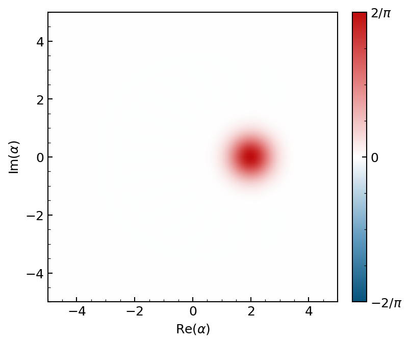
>>> psi = dq.coherent(16, 2.0)
>>> dq.plot.wigner(psi)

plot_wigner_coh

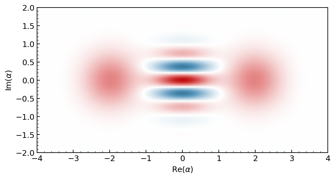
>>> psi = (dq.coherent(16, 2) + dq.coherent(16, -2)).unit()
>>> dq.plot.wigner(psi, xmax=4.0, ymax=2.0, colorbar=False)

plot_wigner_cat

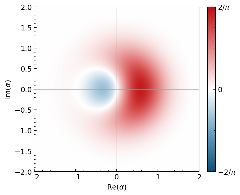
>>> psi = (dq.fock(2, 0) + dq.fock(2, 1)).unit()
>>> dq.plot.wigner(psi, xmax=2.0, cross=True)

plot_wigner_01

>>> psi = dq.coherent(32, [3, 3j, -3, -3j]).sum(0).unit()
>>> dq.plot.wigner(psi, npixels=201, clear=True)

plot_wigner_4legged

wigner.wigner_mosaic

wigner_mosaic(
    states: QArrayLike,
    *,
    n: int = 8,
    nrows: int = 1,
    w: float = 3.0,
    h: float | None = None,
    xmax: float = 5.0,
    ymax: float | None = None,
    vmax: float = 2 / jnp.pi,
    npixels: int = 101,
    cmap: str = "dq",
    interpolation: str = "bilinear",
    cross: bool = False
)

Plot the Wigner function of multiple states in a mosaic arrangement.

Warning

Documentation redaction in progress.

See dq.plot.wigner() for more details.

Examples

>>> psis = [dq.fock(3, i) for i in range(3)]
>>> dq.plot.wigner_mosaic(psis)

plot_wigner_mosaic_fock

>>> n = 16
>>> a = dq.destroy(n)
>>> H = dq.zeros(n)
>>> jump_ops = [a @ a - 4.0 * dq.eye(n)]  # cat state inflation
>>> psi0 = dq.coherent(n, 0)
>>> tsave = jnp.linspace(0, 1.0, 101)
>>> result = dq.mesolve(H, jump_ops, psi0, tsave)
>>> dq.plot.wigner_mosaic(result.states, n=6, xmax=4.0, ymax=2.0)

plot_wigner_mosaic_cat

>>> n = 16
>>> a = dq.destroy(n)
>>> H = a.dag() @ a.dag() @ a @ a  # Kerr Hamiltonian
>>> psi0 = dq.coherent(n, 2)
>>> tsave = jnp.linspace(0, jnp.pi, 101)
>>> result = dq.sesolve(H, psi0, tsave)
>>> dq.plot.wigner_mosaic(result.states, n=25, nrows=5, xmax=4.0)

plot_wigner_mosaic_kerr

wigner.wigner_gif

wigner_gif(
    states: QArrayLike,
    *,
    gif_duration: float = 5.0,
    fps: int = 10,
    w: float = 5.0,
    xmax: float = 5.0,
    ymax: float | None = None,
    vmax: float = 2 / jnp.pi,
    npixels: int = 101,
    cmap: str = "dq",
    interpolation: str = "bilinear",
    cross: bool = False,
    clear: bool = False
) -> Image

Plot a GIF of the Wigner function of multiple states.

Warning

Documentation redaction in progress.

See dq.plot.wigner() and dq.plot.gifit() for more details.

Examples

>>> n = 16
>>> a = dq.destroy(n)
>>> H = dq.zeros(n)
>>> jump_ops = [a @ a - 4.0 * dq.eye(n)]  # cat state inflation
>>> psi0 = dq.coherent(n, 0)
>>> tsave = jnp.linspace(0, 1.0, 1001)
>>> result = dq.mesolve(H, jump_ops, psi0, tsave)
>>> gif = dq.plot.wigner_gif(result.states, fps=25, xmax=4.0, ymax=2.0)

plot_wigner_gif_cat

>>> n = 16
>>> a = dq.destroy(n)
>>> H = a.dag() @ a.dag() @ a @ a  # Kerr Hamiltonian
>>> psi0 = dq.coherent(n, 2)
>>> tsave = jnp.linspace(0, jnp.pi, 1001)
>>> result = dq.sesolve(H, psi0, tsave)
>>> gif = dq.plot.wigner_gif(
...     result.states, gif_duration=10.0, fps=25, xmax=4.0, clear=True
... )

plot_wigner_gif_kerr